Land assessment

Chapter 5 followed the creation and digitisation of the New Zealand Land Resource Inventory and the LADEDA system. The inventory itself was built from stereo aerial photography, geological and soil information, topographic maps and field observations. Its polygons described interpreted land-resource units rather than legal parcels. By the end of the 1970s first-edition coverage comprised about 85,000 mapped units, each carrying codes for rock type, soil, slope, present erosion and vegetation.

The physical inventory was only one part of the system. Land Use Capability, usually shortened to LUC, added an interpreted assessment of what the land could sustain over the long term. The classification took account of the inventory factors together with climate, the effects of past land use and the potential for erosion. It was designed for productive land use and soil conservation rather than for land valuation or statutory zoning.

New Zealand had adapted the LUC approach during the 1950s from a United States soil-conservation system. The national classification used eight broad classes. Limitations increased and versatility decreased from Class 1 to Class 8. Classes 1 to 4 were suitable for arable cropping to varying degrees as well as pastoral, horticultural or forestry uses, while Classes 5 to 7 were not suited to arable cropping but could support pasture or forestry where the physical limitations could be managed. Class 8 was not considered suitable for sustained grazing or production forestry and was associated with catchment protection, conservation or similar non-production uses.

The class number summarised land capability; other attributes explained the limitations. LUC subclasses identified the dominant type of limitation: erosion, wetness, soil or root-zone limitations, or climate. More detailed LUC units then distinguished areas that would respond similarly to management and conservation treatment. The full code therefore combined a broad ranking with information about the kind of physical problem and the local land type.

This structure allowed two areas to share a class while requiring different management. Steep hill country subject to erosion could have a different limitation from low-lying land affected by wetness, even if both fell within the same broad capability class. The extended legends supplied the detail behind the code. Users were expected to read the map and the legend together rather than treat a single number as a complete description of the land.

The classification depended on field and photographic interpretation. Aerial photographs allowed mappers to see landform patterns, vegetation, erosion scars, drainage and other surface characteristics across large areas. Existing soil and geological surveys supplied another part of the evidence. Field visits were needed to check what the imagery and maps could not establish securely and to relate visible patterns to conditions on the ground.

The work was necessarily selective. A national survey at one-inch-to-one-mile scale could not record every soil change, slip, gully or paddock boundary. The mapper had to decide which differences were large and consistent enough to justify a separate unit. Small areas could disappear inside a larger mapped unit, while complex areas might be represented by combined symbols where more than one condition occurred within the mapping scale.

The phrase homogeneous map unit therefore needs to be read in its cartographic sense. It meant that the recorded factors were sufficiently alike for the purpose and scale of the survey, not that every square metre inside the polygon was identical. Later GIS users could zoom into the line until it appeared to divide neighbouring paddocks cleanly, but the original mapping had not been made at that level of detail.

The people doing this work combined several disciplines. Geological and soil knowledge was needed to recognise parent material and soil groups. Land-resource specialists assessed slope, erosion and vegetation. Cartographic staff compiled the boundaries and codes onto base maps. Later digitising and database staff captured the polygons and attached the descriptive information. Much of the surviving published record names system authors and senior specialists more readily than the field and production staff who created the national coverage.

Erosion was built into the NZLRI twice. Present erosion type and severity formed one of the five inventory factors, while susceptibility to future erosion also influenced the LUC assessment. That distinction allowed the mapping to record both what was visible at the time and how vulnerable the land might be under continued or changed use.

The system recognised several forms of erosion because they required different responses. Sheet and rill erosion on cultivated land, soil slips on hill country, gullies, streambank erosion and larger mass-movement processes did not create the same management problem. The mapped severity also mattered. A small area with occasional erosion did not receive the same treatment as land where erosion was widespread or difficult to control.

Soil conservation provided the original practical setting for much of this classification work. Land capability surveys were used at regional and catchment scales, and more detailed surveys supported farm soil and water conservation plans. A farm plan normally began with an inventory and LUC assessment, then set out conservation works or management practices suited to the land. These could include changes to grazing or cultivation, erosion-control planting, water-control work or protection of land that was too unstable for intensive use.

The classification therefore connected mapped evidence with management without turning the map into a legal instruction. A LUC class described physical capability and limitation. It did not determine what a landowner must do, what a council would consent, or whether a particular use was economically attractive. Markets, farm systems, infrastructure and regulation sat outside the physical classification even though they could affect the decision made from it.

The NZLRI gave government agencies and catchment organisations a common way to describe land across large areas. A code for rock, soil, slope, erosion and vegetation could be recorded in the same structured form from Northland to Southland, while the LUC system provided a related assessment of capability. Regional extended legends allowed the classification to be adapted to local combinations of geology, climate and landform rather than forcing every landscape into identical detailed units.

That regional structure later created work when users wanted national consistency. Below the broad class and subclass levels, the original LUC units formed regional classifications rather than one seamless national scheme. Different regions had their own units and extended legends. Correlation between them required expert interpretation, because a locally defined unit reflected the conditions and mapping history of that region.

The national inventory was still useful precisely because the broad structure remained recognisable. Users could distinguish highly versatile land from land with severe erosion, soil, wetness or climate limitations and then move into the regional legend for detail. The system supported comparison without pretending that a hill-country land unit in Gisborne was identical to one in Otago because both carried the same broad class number.

The mapping also supplied a base for later derived information. Pastoral or forestry potential, land-use recommendations and other interpretations could be related back to the same physical inventory. Once the polygons had been digitised, those relationships could be stored and selected systematically. The computer made retrieval easier, but the analytical value still came from the classification work attached to each polygon.

Many users continued to obtain NZLRI information as printed maps. Paper worksheets and extended legends remained the main way the information was distributed for much of the period. A planner, catchment officer or consultant could work from a printed sheet showing the coded map units and then use the accompanying legend to interpret the rock, soil, slope, erosion, vegetation and LUC information. The GIS sat behind production and analysis while paper remained the practical interface for many users. Digital geography had arrived, but for plenty of people its user interface was still a folded sheet, a legend and enough desk space to spread them out.

This arrangement suited organisations that needed the information without maintaining their own GIS. A regional office could request a particular map or use the standard worksheet series without buying specialist hardware and software. Where a different thematic view was needed, the database could support a new plot and the result could again be delivered on paper. Digital storage therefore widened the range of outputs before it changed the way every user accessed them.

The separation also affected how errors and revisions travelled. A correction made to the maintained database could be incorporated into later plots, but an older worksheet already sitting in an office drawer did not update itself. Users could therefore be working from different editions or survey dates without the difference being obvious from the appearance of the map alone. Extended legends, edition information and source dates were part of using the data properly.

Regional planning used the same material at a broader scale. Agencies could compare the distribution of capability classes, erosion limitations or other land-resource characteristics across catchments or districts and identify areas requiring more detailed investigation. The national inventory was suitable for screening and regional assessment because it had been compiled consistently enough to support those comparisons. It was not a substitute for the detailed survey needed when a decision depended on conditions within a particular property or development site.

At farm scale, the land-capability approach became more specific. Soil and water conservation planning used land inventory and capability assessments to divide a property according to erosion risk, wetness, soil limitations and other constraints. Conservation staff could then recommend different treatment for different parts of the farm rather than assume one management practice suited the whole property.

The map might separate flatter cultivable land from steeper pastoral land, erosion-prone faces and areas better kept under protective vegetation. The classes described different land capabilities and management constraints. A lower-capability unit could still have a productive role if managed within its physical limits, while Class 8 land could be valuable for catchment protection, biodiversity, recreation or water yield. The classification described capability for sustained production, not the total value of a place.

Catchment authorities and later regional councils continued preparing detailed land-capability maps and soil-conservation plans after the national first-edition programme had finished. These local surveys worked at finer scales than the national NZLRI and could record variation that the regional dataset necessarily generalised. A farm-scale plan and the national inventory therefore served related but different purposes.

This difference in scale would later become easy to overlook in GIS. A national polygon could be clipped neatly to a farm boundary and displayed beside detailed property information. That did not make the national land-resource mapping a farm survey. The operation changed the extent of the file, not the scale at which the original information had been collected.

The same classification logic was adapted for urban planning during the 1980s. M. R. Jessen’s 1987 *Urban Land Use Capability Survey Handbook* documented a system developed for land evaluation at the more detailed scales required for urban development. The work drew on the LUC tradition but focused on constraints relevant to settlement, infrastructure and hazard rather than on agricultural production alone.

The handbook acknowledged earlier urban capability surveys and the contribution of catchment-authority staff. Bob Cathcart of the Northland Catchment Commission was credited with preparing some of the earliest New Zealand urban LUC surveys and demonstrating their use in urban planning. Staff from twelve catchment authorities commented during development of the handbook, and Palmerston North City Corporation also contributed to the final review.

Later institutional histories record urban LUC use by councils including Whangarei and Palmerston North for planning and hazard mapping. At urban scales, questions about slope stability, flooding, drainage, erosion and ground conditions could affect the suitability of land for development. A capability map gave planners a way to organise those physical constraints spatially rather than relying on separate reports with different boundaries.

Urban LUC was used for particular planning and assessment tasks. Its documented use by a few councils is enough to show how the land-capability approach travelled into another field. The method was being adapted to the scale and decisions of the user rather than applied unchanged from a rural national map.

The first-edition NZLRI worksheets were digitised between 1977 and 1980, and the database was managed through the LADEDA environment before moving into ARC/INFO in the late 1980s. Chapter 5 covered that conversion in detail. For users of land-resource information, the operational change was that the same mapped units could now be selected by their attributes and plotted in different combinations.

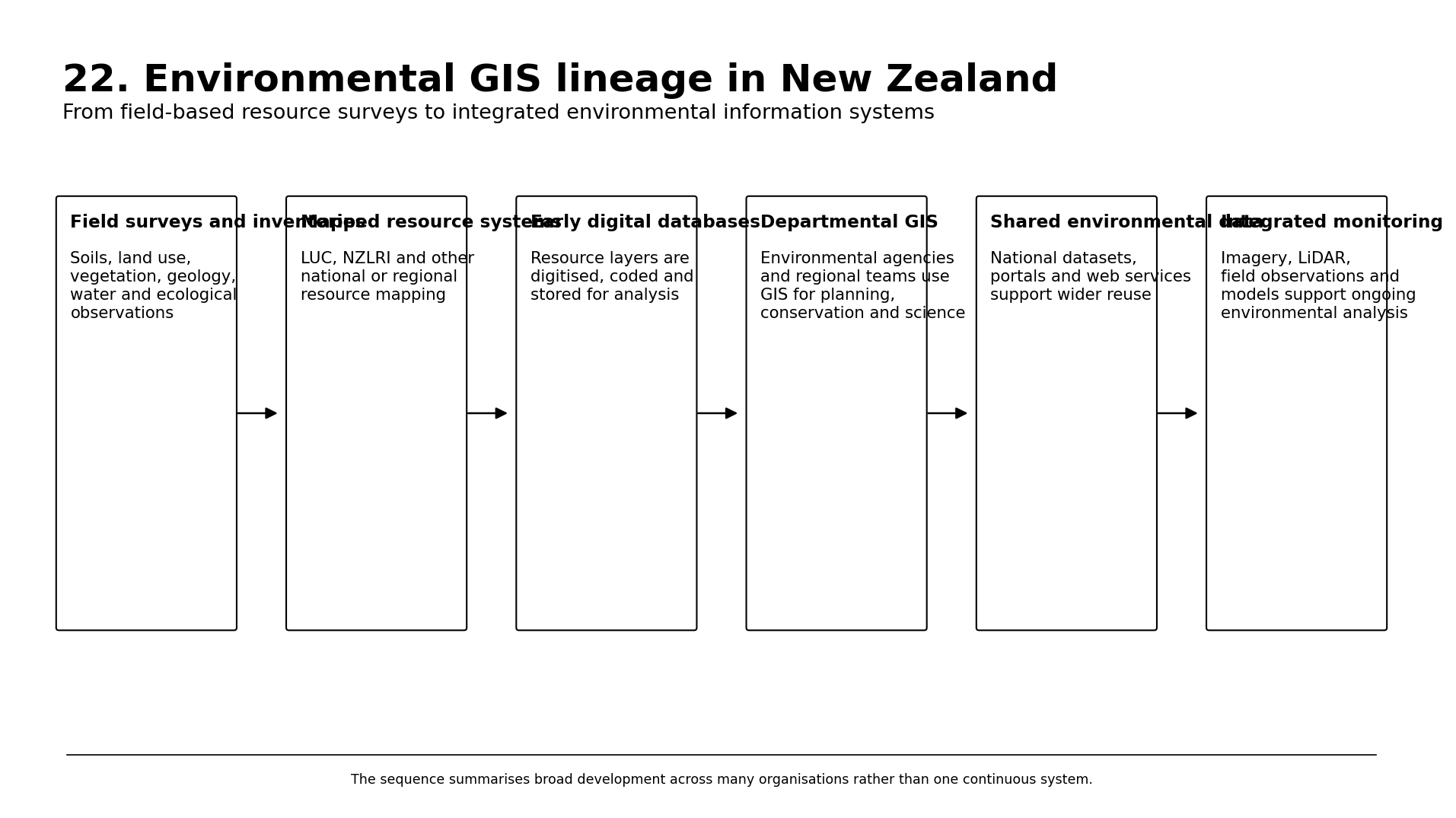
Image source · EX22-V01

NZ GIS History project, 2026. Simplified explanatory synthesis.

A request no longer had to begin with a cartographer manually compiling every relevant unit from several sheets. A database query could identify polygons sharing an erosion class, slope range, soil grouping or LUC category, subject to the coding available in the data. The resulting map could be produced for a planning or research task without altering the underlying national record.

The digital database also separated the inventory from its standard printed presentation. One worksheet displayed a particular set of symbols and labels because paper space was limited. In GIS the user could emphasise one attribute and suppress another, combine the polygons with administrative boundaries or compare them with other spatial datasets. The national land-resource units became inputs to other analyses rather than remaining only the content of the original worksheet series.

None of this changed the origin of the polygons. A query could retrieve every unit coded with a particular erosion limitation very quickly, but the answer still depended on field mapping and classification carried out years earlier. A clean thematic plot could make the selection look current even when the underlying observation was not. As GIS made reuse easier, the age and provenance of the data became more relevant rather than less.

Between 1987 and 1990 the NZLRI mapping was converted from the old 1:63,360 framework to 1:50,000. Chapter 5 followed the production work: polygon boundaries were checked against aerial photography and newer topographic information, including coastlines, lakes, trig points and geographic control. The conversion did more than rescale a printed map. It placed the land-resource geometry into the metric national mapping framework being used more widely across government and GIS.

For later users, this made comparison with the NZMS260 topographic series and other 1:50,000 datasets easier. Boundaries that had been compiled against older base information could be adjusted where newer photography or mapping showed a mismatch. The thematic interpretation was retained unless the land-resource evidence itself justified a change.

Several regions were also remapped as second editions, including Northland, Wellington, Marlborough and Gisborne-East Coast, with some work extending into the 1990s. These revisions used newer resource information and more detailed 1:50,000 mapping where available. The national dataset therefore became a mixture of first- and second-edition work rather than one survey frozen permanently in 1979.

This mixed history is visible in later use. Some regions contain newer field interpretation and revised legends than others. A national GIS layer can make those differences difficult to see because all polygons use the same display technology. The metadata and regional documentation remain necessary for understanding when and how a particular area was mapped.

By the mid-1990s funding for regional-scale NZLRI remapping had largely ceased. Institutional histories later described the national database as static in some respects and acknowledged that parts of the information had become outdated. Land cover changes, new erosion, changing drainage, forestry, subdivision and revised soil or geological knowledge could all alter conditions after the original survey.

The problem affected different attributes differently. Rock type changed slowly and could remain useful for decades, while vegetation and erosion could change substantially over much shorter periods. A polygon could therefore contain a mixture of relatively durable physical information and observations tied closely to the date of survey. Treating the whole record as equally current would hide that distinction.

Digitised data still required maintenance. It made updates technically easier once revised information existed, but someone still had to fund new mapping, field checks and interpretation. A national database could survive organisational restructuring and software changes while gradually becoming less current in places where no new survey work was carried out.

The institutional home also changed. Water and Soil functions passed through the restructuring of the late 1980s and early 1990s, and Landcare Research inherited the national land-resource database during Crown Research Institute formation. The data later became part of nationally significant science collections and eventually moved into modern online distribution systems. Those later access changes rested on the same polygons and classifications built through the earlier survey programme.

The history of NZLRI is a useful warning against treating a GIS polygon as a simple fact. The line around a land-resource unit records a professional judgement made from aerial photography, maps, field observations and classification standards at a particular scale and time. Its attributes contain both observed or mapped physical factors and an interpreted capability assessment. The digital database preserves those decisions with great consistency.

That consistency is useful. It allows a national analysis to apply the same fields and broad classification logic across large areas. It also allows an old judgement to be repeated very efficiently if the user ignores the survey date, scale or regional legend. The quality of the GIS output remains tied to the quality and suitability of the resource mapping beneath it.

NZLRI and LUC continued to be used because they provided a national framework that few later projects could afford to recreate from the beginning. Their long life also reflects the cost of replacing nationwide field-based mapping. Building a new layer with finer pixels or newer software is straightforward compared with sending trained people across the country to reinterpret soils, erosion, slope, rock and vegetation consistently.

By the 1990s New Zealand therefore had something more durable than a set of land-capability sheets. It had a national spatial record assembled from field science, aerial-photo interpretation and classification, carried through early GIS and into later commercial systems. The computer changed how the information could be stored, queried and combined. The land-resource survey determined what the information meant.

Forestry created another large demand for digital spatial information through inventories, stand boundaries, terrain and operational planning. Forestry brought different data, different scales and different business decisions, but it inherited the same basic problem: converting a mapped landscape into information that could be maintained and used repeatedly.